SmartPath - Customer Data

Exploring the fictional dataset Customer Data, provided during SmartPath Data Analyst Bootcamp

On this page

• Setup
  • Libraries
  • Options
  • Variables
  • Inspect Dataset
  • Explore Categorical Variables
  • Explore Numerical Variables
    • Explore Relationships

Setup

We’ll be using the tidyverse library, as well as some useful packages for a quick data inspection such as summarytools and DataExplorer

Libraries

library(tidyverse)

── Attaching core tidyverse packages ──────────────────────── tidyverse 2.0.0 ──
✔ dplyr     1.1.4     ✔ readr     2.1.5
✔ forcats   1.0.0     ✔ stringr   1.5.1
✔ ggplot2   3.5.1     ✔ tibble    3.2.1
✔ lubridate 1.9.3     ✔ tidyr     1.3.1
✔ purrr     1.0.2     
── Conflicts ────────────────────────────────────────── tidyverse_conflicts() ──
✖ dplyr::filter() masks stats::filter()
✖ dplyr::lag()    masks stats::lag()
ℹ Use the conflicted package (<http://conflicted.r-lib.org/>) to force all conflicts to become errors

library(DataExplorer)
library(summarytools)

Attaching package: 'summarytools'

The following object is masked from 'package:tibble':

    view

Options

I’m not good with scientific notation. It’s hard to read. So let’s turn it off by setting the threshold to a high value. While we’re at it, we can also set the amuont of significance digits.

options(scipen = 999, digits = 2)

Variables

df <- read.csv('customer_data.csv') |> 
  as_tibble()

Inspect Dataset

All set, let’s check out the dataset (no pun intended).

df

# A tibble: 2,240 × 9
      ID Year_Birth Education  Income Dt_Customer Recency NumWebPurchases
   <int>      <int> <chr>       <int> <chr>         <int>           <int>
 1  5524       1957 Graduation  58138 9/4/2012         58               8
 2  2174       1954 Graduation  46344 3/8/2014         38               1
 3  4141       1965 Graduation  71613 8/21/2013        26               8
 4  6182       1984 Graduation  26646 2/10/2014        26               2
 5  5324       1981 PhD         58293 1/19/2014        94               5
 6  7446       1967 Master      62513 9/9/2013         16               6
 7   965       1971 Graduation  55635 11/13/2012       34               7
 8  6177       1985 PhD         33454 5/8/2013         32               4
 9  4855       1974 PhD         30351 6/6/2013         19               3
10  5899       1950 PhD          5648 3/13/2014        68               1
# ℹ 2,230 more rows
# ℹ 2 more variables: NumStorePurchases <int>, NumWebVisitsMonth <int>

glimpse(df)

Rows: 2,240
Columns: 9
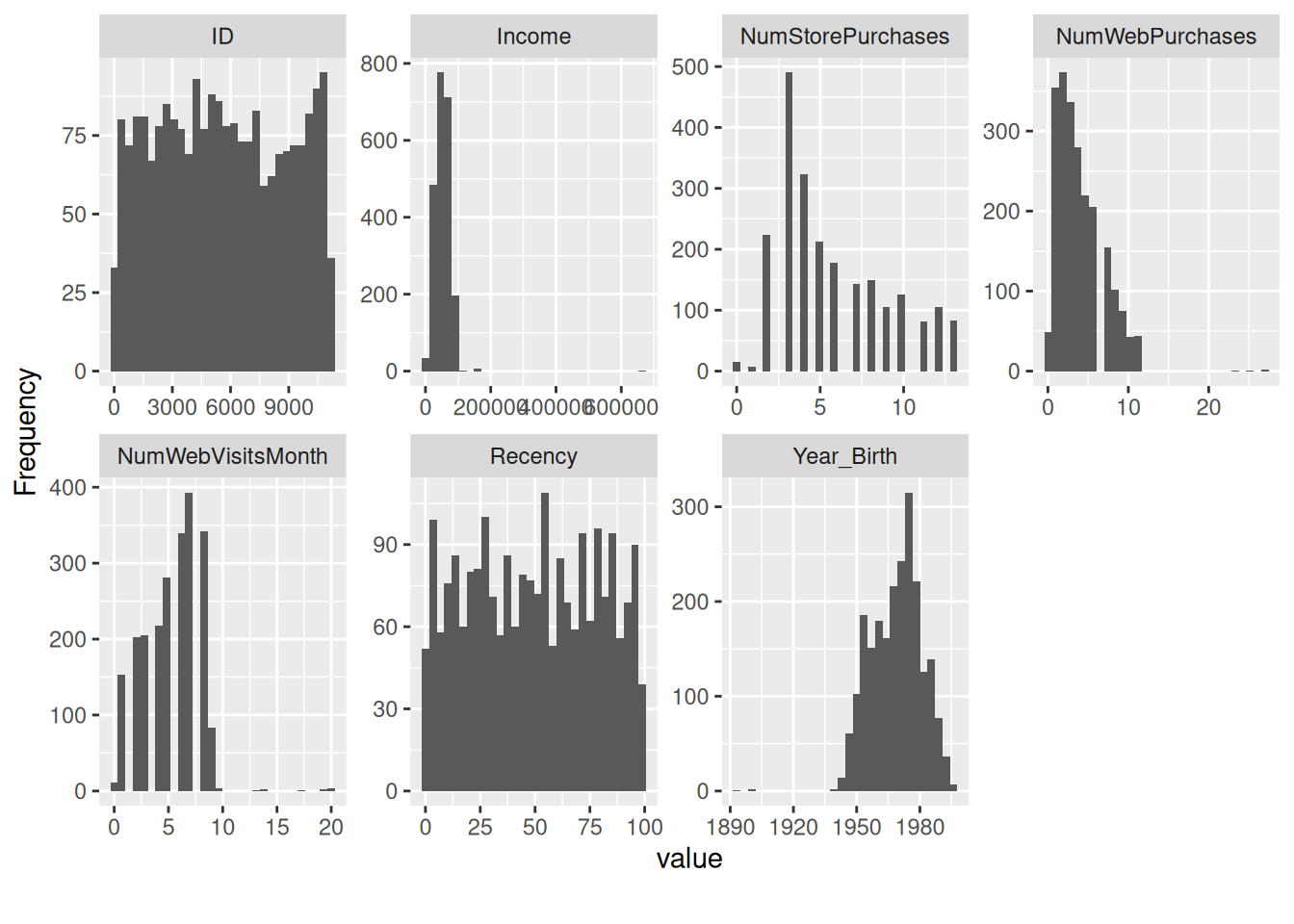
$ ID                <int> 5524, 2174, 4141, 6182, 5324, 7446, 965, 6177, 4855,…
$ Year_Birth        <int> 1957, 1954, 1965, 1984, 1981, 1967, 1971, 1985, 1974…
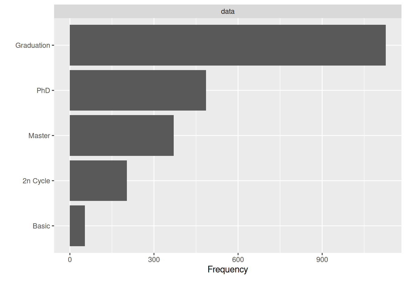
$ Education         <chr> "Graduation", "Graduation", "Graduation", "Graduatio…
$ Income            <int> 58138, 46344, 71613, 26646, 58293, 62513, 55635, 334…
$ Dt_Customer       <chr> "9/4/2012", "3/8/2014", "8/21/2013", "2/10/2014", "1…
$ Recency           <int> 58, 38, 26, 26, 94, 16, 34, 32, 19, 68, 11, 59, 82, …
$ NumWebPurchases   <int> 8, 1, 8, 2, 5, 6, 7, 4, 3, 1, 1, 2, 3, 6, 1, 7, 3, 4…
$ NumStorePurchases <int> 4, 2, 10, 4, 6, 10, 7, 4, 2, 0, 2, 3, 8, 5, 3, 12, 3…
$ NumWebVisitsMonth <int> 7, 5, 4, 6, 5, 6, 6, 8, 9, 20, 7, 8, 2, 6, 8, 3, 8, …

At a glance, we can spot several problems with this dataset:

1. Dt_Customer should’ve been a date format. from the first few rows, the date seems to be complete, so let’s try parsing it.

df$Dt_Customer |> 
  mdy() |> 
  head()

[1] "2012-09-04" "2014-03-08" "2013-08-21" "2014-02-10" "2014-01-19"
[6] "2013-09-09"

There is no error, fortunately, so we can apply it right away.

df$Dt_Customer <- df$Dt_Customer |> 
  mdy()

2. Year_Birth is a bit tricky. It’s actually an incomplete date, but we can’t convert it to date format either because we need the month and days too. We can set everything as January the 1st, but that would be misleading. Integers would also be inaccurate because it’s not really a number, we aren’t supposed to perform arithmetic operations on it. However, I believe it’s the most ideal type. So we can leave it as it is.

Now let’s further explore the variables. We’ll start with the categorical since there is only one.

Explore Categorical Variables

freq(df)

Variable(s) ignored: ID, Year_Birth, Income, Dt_Customer, Recency

Frequencies  
df$Education  
Type: Character  

                   Freq   % Valid   % Valid Cum.   % Total   % Total Cum.
---------------- ------ --------- -------------- --------- --------------
        2n Cycle    203      9.06           9.06      9.06           9.06
           Basic     54      2.41          11.47      2.41          11.47
      Graduation   1127     50.31          61.79     50.31          61.79
          Master    370     16.52          78.30     16.52          78.30
             PhD    486     21.70         100.00     21.70         100.00
            <NA>      0                               0.00         100.00
           Total   2240    100.00         100.00    100.00         100.00

df$NumWebPurchases  
Type: Integer  

              Freq   % Valid   % Valid Cum.   % Total   % Total Cum.
----------- ------ --------- -------------- --------- --------------
          0     49     2.188          2.188     2.188          2.188
          1    354    15.804         17.991    15.804         17.991
          2    373    16.652         34.643    16.652         34.643
          3    336    15.000         49.643    15.000         49.643
          4    280    12.500         62.143    12.500         62.143
          5    220     9.821         71.964     9.821         71.964
          6    205     9.152         81.116     9.152         81.116
          7    155     6.920         88.036     6.920         88.036
          8    102     4.554         92.589     4.554         92.589
          9     75     3.348         95.938     3.348         95.938
         10     43     1.920         97.857     1.920         97.857
         11     44     1.964         99.821     1.964         99.821
         23      1     0.045         99.866     0.045         99.866
         25      1     0.045         99.911     0.045         99.911
         27      2     0.089        100.000     0.089        100.000
       <NA>      0                              0.000        100.000
      Total   2240   100.000        100.000   100.000        100.000

df$NumStorePurchases  
Type: Integer  

              Freq   % Valid   % Valid Cum.   % Total   % Total Cum.
----------- ------ --------- -------------- --------- --------------
          0     15      0.67           0.67      0.67           0.67
          1      7      0.31           0.98      0.31           0.98
          2    223      9.96          10.94      9.96          10.94
          3    490     21.88          32.81     21.88          32.81
          4    323     14.42          47.23     14.42          47.23
          5    212      9.46          56.70      9.46          56.70
          6    178      7.95          64.64      7.95          64.64
          7    143      6.38          71.03      6.38          71.03
          8    149      6.65          77.68      6.65          77.68
          9    106      4.73          82.41      4.73          82.41
         10    125      5.58          87.99      5.58          87.99
         11     81      3.62          91.61      3.62          91.61
         12    105      4.69          96.29      4.69          96.29
         13     83      3.71         100.00      3.71         100.00
       <NA>      0                               0.00         100.00
      Total   2240    100.00         100.00    100.00         100.00

df$NumWebVisitsMonth  
Type: Integer  

              Freq   % Valid   % Valid Cum.   % Total   % Total Cum.
----------- ------ --------- -------------- --------- --------------
          0     11     0.491          0.491     0.491          0.491
          1    153     6.830          7.321     6.830          7.321
          2    202     9.018         16.339     9.018         16.339
          3    205     9.152         25.491     9.152         25.491
          4    218     9.732         35.223     9.732         35.223
          5    281    12.545         47.768    12.545         47.768
          6    340    15.179         62.946    15.179         62.946
          7    393    17.545         80.491    17.545         80.491
          8    342    15.268         95.759    15.268         95.759
          9     83     3.705         99.464     3.705         99.464
         10      3     0.134         99.598     0.134         99.598
         13      1     0.045         99.643     0.045         99.643
         14      2     0.089         99.732     0.089         99.732
         17      1     0.045         99.777     0.045         99.777
         19      2     0.089         99.866     0.089         99.866
         20      3     0.134        100.000     0.134        100.000
       <NA>      0                              0.000        100.000
      Total   2240   100.000        100.000   100.000        100.000

I honestly didn’t expect the 3 numerical variables to show up. After I think about it, it kinda makes sense, because they’re integers, so they aren’t continuous, they discrete. It may be useful to inspect their frequency to spot outliers, but for now we’ll focus on Education.

df$Education |> freq()

Frequencies  
df$Education  
Type: Character  

                   Freq   % Valid   % Valid Cum.   % Total   % Total Cum.
---------------- ------ --------- -------------- --------- --------------
        2n Cycle    203      9.06           9.06      9.06           9.06
           Basic     54      2.41          11.47      2.41          11.47
      Graduation   1127     50.31          61.79     50.31          61.79
          Master    370     16.52          78.30     16.52          78.30
             PhD    486     21.70         100.00     21.70         100.00
            <NA>      0                               0.00         100.00
           Total   2240    100.00         100.00    100.00         100.00

df$Education |> plot_bar()

No serious problems spotted. No missing values, no weird values. The distribution also seems ‘normal’. The frequency increases as the education goes up, except for the PhD. We could guess that the customers are mostly from well-educated backgrounds.

Now let’s explore the numerical variables.

Explore Numerical Variables

descr(df, stats=c('n.valid', 'pct.valid', 'mean', 'min', 'q1', 'q3', 'max'))

Non-numerical variable(s) ignored: Education, Dt_Customer

Descriptive Statistics  
df  
N: 2240  

                        ID      Income   NumStorePurchases   NumWebPurchases   NumWebVisitsMonth
--------------- ---------- ----------- ------------------- ----------------- -------------------
        N.Valid    2240.00     2216.00             2240.00           2240.00             2240.00
      Pct.Valid     100.00       98.93              100.00            100.00              100.00
           Mean    5592.16    52247.25                5.79              4.08                5.32
            Min       0.00     1730.00                0.00              0.00                0.00
             Q1    2827.50    35284.00                3.00              2.00                3.00
             Q3    8428.50    68557.00                8.00              6.00                7.00
            Max   11191.00   666666.00               13.00             27.00               20.00

Table: Table continues below

 

                  Recency   Year_Birth
--------------- --------- ------------
        N.Valid   2240.00      2240.00
      Pct.Valid    100.00       100.00
           Mean     49.11      1968.81
            Min      0.00      1893.00
             Q1     24.00      1959.00
             Q3     74.00      1977.00
            Max     99.00      1996.00

df |> plot_histogram()

Nearly no missing values, perfect. The only missing values are within Income, which are only about 2%. We could drop the rows, but we don’t need to for now. The valid data in the other columns can still provide aid to other analysis.

I’m interested to why they are missing, though. We have 2 data that we could analyze it with: Year_Birth and Education. Maybe older people tend to be sensitive about their income, so they leave it empty. Or maybe it’s the younger people that do! (who knows?).

Unfortunately, I think 2% is too small of a sample to get reliable result. So let’s just leave it as it is.

Explore Relationships

With all these numeric variables, there’s various relationships we could investigate. As starters, let’s draw up a correlation matrix to see a broad overview. We’ll remove ID since it’s irrelevant.

df_numeric <- df |> 
  select(!ID)
plot_correlation(df_numeric, type = 'continuous', maxcat = 0, cor_args =  list("use" = "pairwise.complete.obs"))